My girlfriend is currently working on her master’s thesis, which is, in parts, about Open Source software projects.
Recently, we were discussing the typical distribution of people’s level of involvement.
Of course, I was interested how this looks for GNU Radio.
I would say that with GNU Radio we can distinguish between technical code contributions and community support.
Since, there aren’t a lot of non-technical, documentation-only changes in git, I think that the git history might be a good indicator for technical involvement.
Summarizing the commits for 2015 with
git shortlog -sn --no-merges --after 2015-01-01 origin/next | tr '\t' ','
and plotting the Top 20, we get the following distribution.
Note, that Tom has so many commits even excluding merges.
Regarding community support, the mailing list might be a good starting point.
On the list, people mainly provide help with GNU Radio, out-of-tree modules, and radio in general.
Discussions about implementation details of GNU Radio are very seldom, i.e., it’s a typical user mailing list.
Copying the mails from 2015 in a maildir folder and running
#!/usr/bin/env python

import mailbox

mbox = mailbox.Maildir("/home/basti/mail/.gnuradio")
for message in mbox:
        print message["from"]
Using vim to reduce the entries to email addresses and counting occurrences with uniq -c I got
which quantifies Marcus Mueller’s total domination of the list :-)
Yesterday, I started off fixing the unit tests of the GNU Radio ZigBee module, which were broken since the CSS phy got merged.
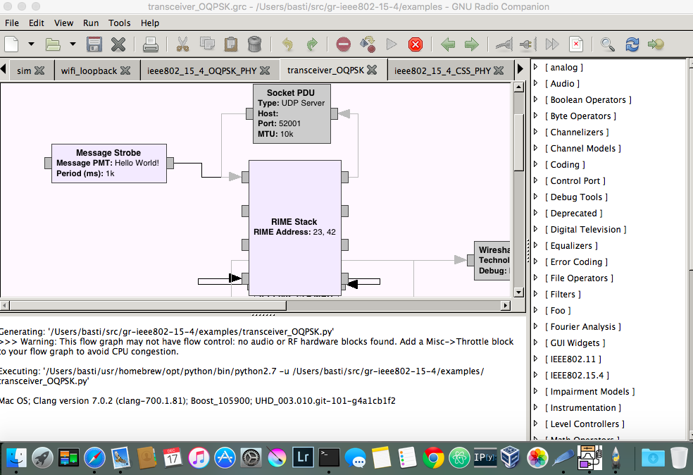
However, opening the flow graphs in GNU Radio Companion, I soon realized that the module didn’t work at all on my Mac. (Whoot?!?)
I immediately checked on a Linux machine and—luckily—it worked perfectly fine.
The symptoms on OS X were rather strange: I started the flow graph in GRC and absolutely nothing happened.
It looked like it would run, only that no window appeared and no error message was shown.
At first, I thought that GRC hides some errors and started the flow graph in a terminal, but it showed the exact same behaviour.
read more
Sometimes, it makes me sad to see so many ugly plots in papers and student reports—and I’m not talking about things that could be regarded as subjective, like an aversion against pie charts, 3D bar plots, or the rainbow color palette.
I’m talking about rescaled pixel graphics with unreadable axes labels, which—I would argue—are objectively crap.
As a student/researcher/engineer, who communicates his results mainly with graphs, it is worth to sit down for an hour and get this right—once and forever.
It is really not too hard, the work flow to generate a nice graph is
- determine the graph’s final size
- create the graph in correct size, using the font family and font size of the main document
- insert the graph in the document without rescaling
OK, so let’s do this.
Determine the Final Size
To determine the plots final size in the document, I created a placeholder PDF with nothing but a brown background.
Its size doesn’t matter, it will be rescaled to fit the adjusted width.
(This is, btw, exactly what we want to avoid for our final graph.)
Then, insert the placeholder PDF in the document.
If you want it to fill one column, this will be something like
\begin{figure}
    \includegraphics[width=\columnwidth]{placeholder}
    \caption{This is a placeholder to measure the width of a plot. Its with is set to \texttt{columnwidth}.}
\end{figure}
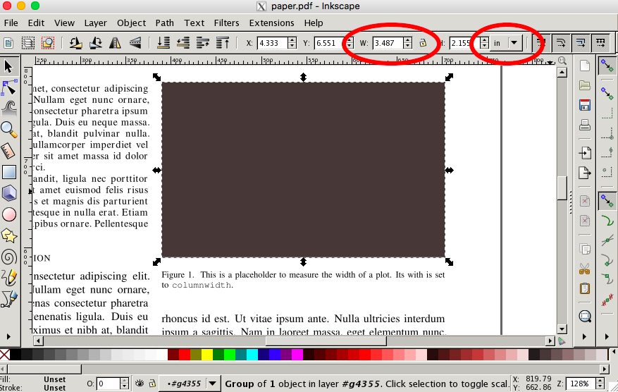
Generate the PDF and open it in Inkscape.
When you double click on you placeholder you can see its dimensions in the top bar.
Since, Matplotlib measures sizes in inches, it’s easiest to switch to inches.
read more
In the last quarter, I helped some students who worked on a feasibility study that included near field measurements.
To be honest, I have absolutely no idea what’s going on in the near field, but according to Wikipedia some fancy stuff happens.
The students used my WiFi transceiver and experimented with very small distances.
Using a center frequency of 5.62GHz and a VERT 2450 antenna with a height of about 17cm, the reactive near field spans about 18.8cm.
$$
\mbox{reactive} = 0.62 \cdot \sqrt{\dfrac{D^3}{\lambda}}
$$
c = 3e8
f = 5.62e9
wavelength = c / f

D = .17
reactive = .62 * (D**3/wavelength)**.5

Out[7]: 0.18809298643667358
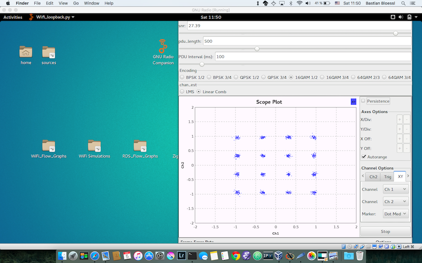
In a first experiment they moved the antenna around while watching the constellation plot.
It just went crazy when the antennas were in the reactive near field.
At first, I thought that we see clipping effects as the receiver overdrives, but we double-checked and asserted that the power level was still fine.
The students also did some quick measurement that showed reasonable results.
That might not be rocket science, but I found it very cool to play with stuff from textbooks in a real experiment in our lab.
Was quite a while since I last looked into GNU Radio’s Performance Counters [1].
Turns out, they changed quite a bit.
The current implementation is no longer based on the strange ICE framework, but uses Apache Thrift.
I guess there are good reasons for this, but the user experience, certainly, was not the driving force :-)
As far as I see, GNU Radio requires Thirft 0.9.2, which is not even part of the most recent Ubuntu release.
Since I didn’t find a PPA, I installed packages that are seemingly from one of the developers.
Once Thrift is installed, you should run cmake again and assert that thrift is explicitly listed in the activated components, since only gr-ctrlport does not do anything.
-- ######################################################
-- # Gnuradio enabled components
-- ######################################################
--   * python-support
--   * testing-support
--   * volk
--   * gnuradio-runtime
--   * gr-ctrlport
--   * * thrift      <----- !!!!
--   * gr-blocks
--   * gnuradio-companion
--   * gr-fec
[...]
During the last weeks I advised some students that worked on building a simulation framework for my WiFi transceiver.
It is really surprising how many students have problems using a compiler to install software that is not in the package manager.
To give them a head start, I created a virtual machine image based on Ubuntu Gnome 15.10 with a lot of software preinstalled.
It’s mainly a development environment with everything compiled from git and installed in the users home; ready to adapt the gitconfig, hack, and make pull requests.
The VM is in OVA format, which is supposed to be understood by all main appliances.
However, I only tested VirtualBox.
(One student told me that he had to disable some hyper visor option to get it running.)
You can download the image here.
The login is user: project and password: project.
Recently, I set up some simulations for my WiFi transceiver.
There will be some follow-ups describing the simulation framework and some results, but in this post I wanted to capture things I stumbled upon while setting up the simulations.
Generating Random Messages
The first thing was to generate WiFi frames with a random payload.
The WiFi transmitter expects PMTs (i.e., GNU Radio’s Polymorphic Message Type) as input, which can be produced with the Message Source block.
I wanted the payload to be pseudo random and derived from the current repetition to ensure reproducibility.
After some fiddling in Python I came up with
pmt.intern("".join([chr(random.randint(0,255)) for x in (lambda: (random.seed(repetition) == None) and range(pdu_len-24))()]))
It seeds the Python random number generator with the current repetition and creates a PMT string with pdu_len random bytes.
(The -24 accounts for WiFi headers like MAC address and sequence number.)
It looks a bit over complicated, but it works.
Let me know if you know of a simpler way to do this.
Note, that this code is executed when the block is initialized.
That means that it will always send the same message during a repetition, but produce different messages in different repetitions.
read more
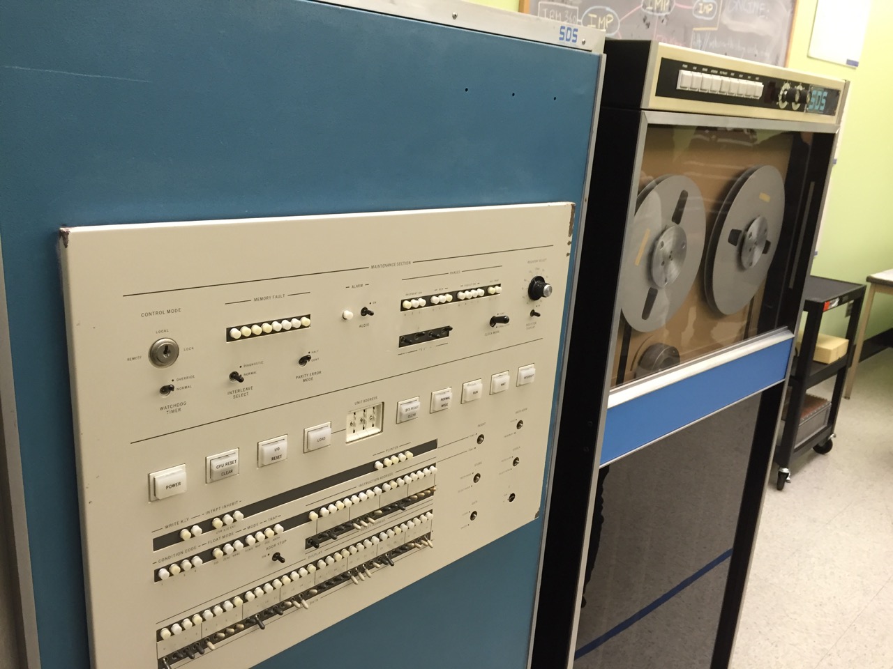
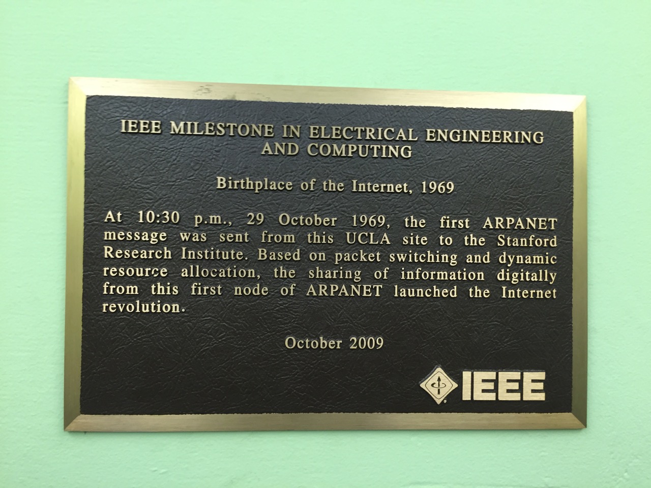
I already knew that UCLA is considered to be the birthplace of the Internet.
Turns out they also kept the room where everything started and it’s only down the floor from our lab.
Fortunately, Mario Gerla has access and showed us around, telling stories from back then.
It was really amazing.
The Interface Message Processor (IMP) is the big refrigerator-sized box with the crazy wiring, which was basically the first modem.
read more
Today, I got an email from Google Scholar, notifying me that I have a new citation to my article.
Usually, I have a look to checkout the context of the reference.
The article from today was great.
It was so great, I could have written it myself… and indeed, large parts I did!
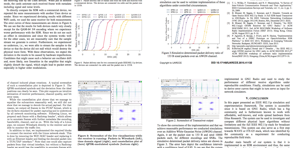
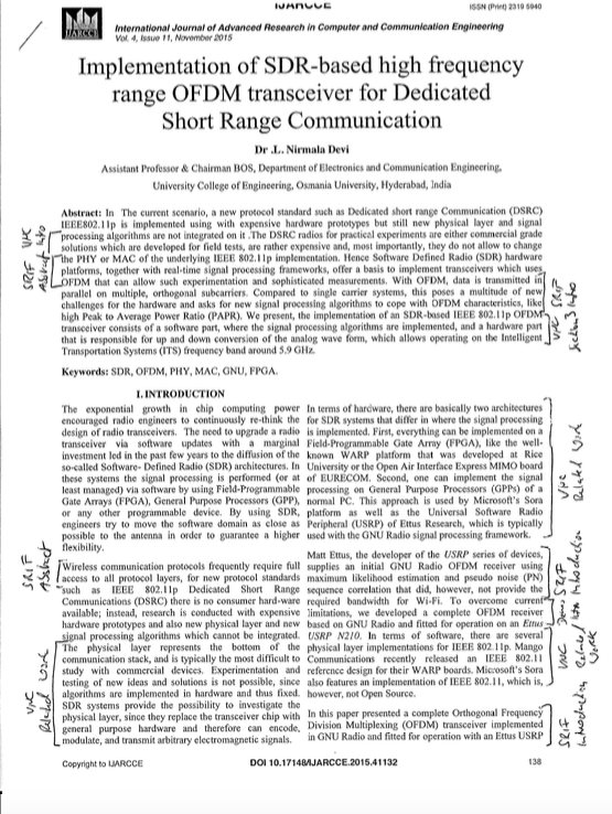
The paper, is basically a bad remix of my work.
She even copied my graphs and claims that she implemented my WiFi transceiver. WTF?!?
I wonder if I should put the paper on my publications list :-)
Here is a comparison of my stuff (left) and hers (right).
Also the text is very similar. We annotated on some pages where we found verbatim copies. Here is an example
Fun fact: She even messed up removing hyphens when words were divided in my document.
Academia at its best…
Having a handy simulation framework for my WiFi transceiver, I used it for a quick simulation study for the sensitivity of the frame detection block.
Frame detection in WiFi is usually implemented based on autocorrelation, as the short preamble is comprised of a pattern that repeats ten times.
Having a noisy signal, the question is at which autocorrelation threshold to trigger frame detection.
This is of course a trade-off between missed frames (if not triggered) and computational overhead (when triggered on noise).
In my implementation, I calculate the autocorrelation coefficient, i.e., normalize the autocorrelation with the power of the signal.
(Actually, I use a slightly larger window for the power then for the autocorrelation, but that’s not important here.)
Running the simulations with 435 byte frames BPSK 1/2, I get the following graph.
I would say 0.56 is a pretty good value here.
Therefore, I added a sensitivity parameter to the WiFi physical layer block and set its default value of 0.56.
The code is already on Github.
Of course an analytical study, considering also impairments like frequency offset is still to do, but I think it’s a good starting point.

