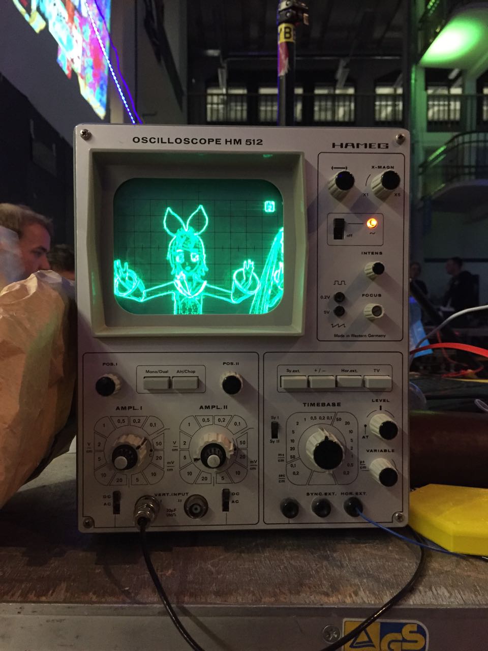
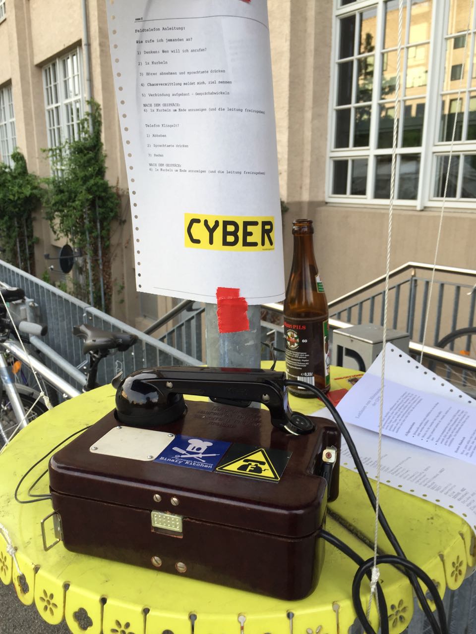
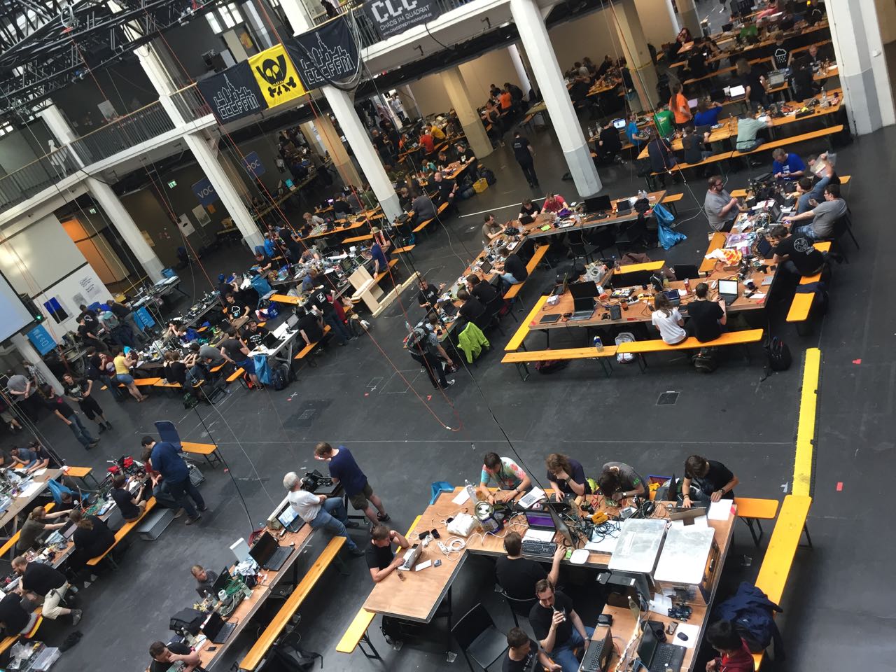
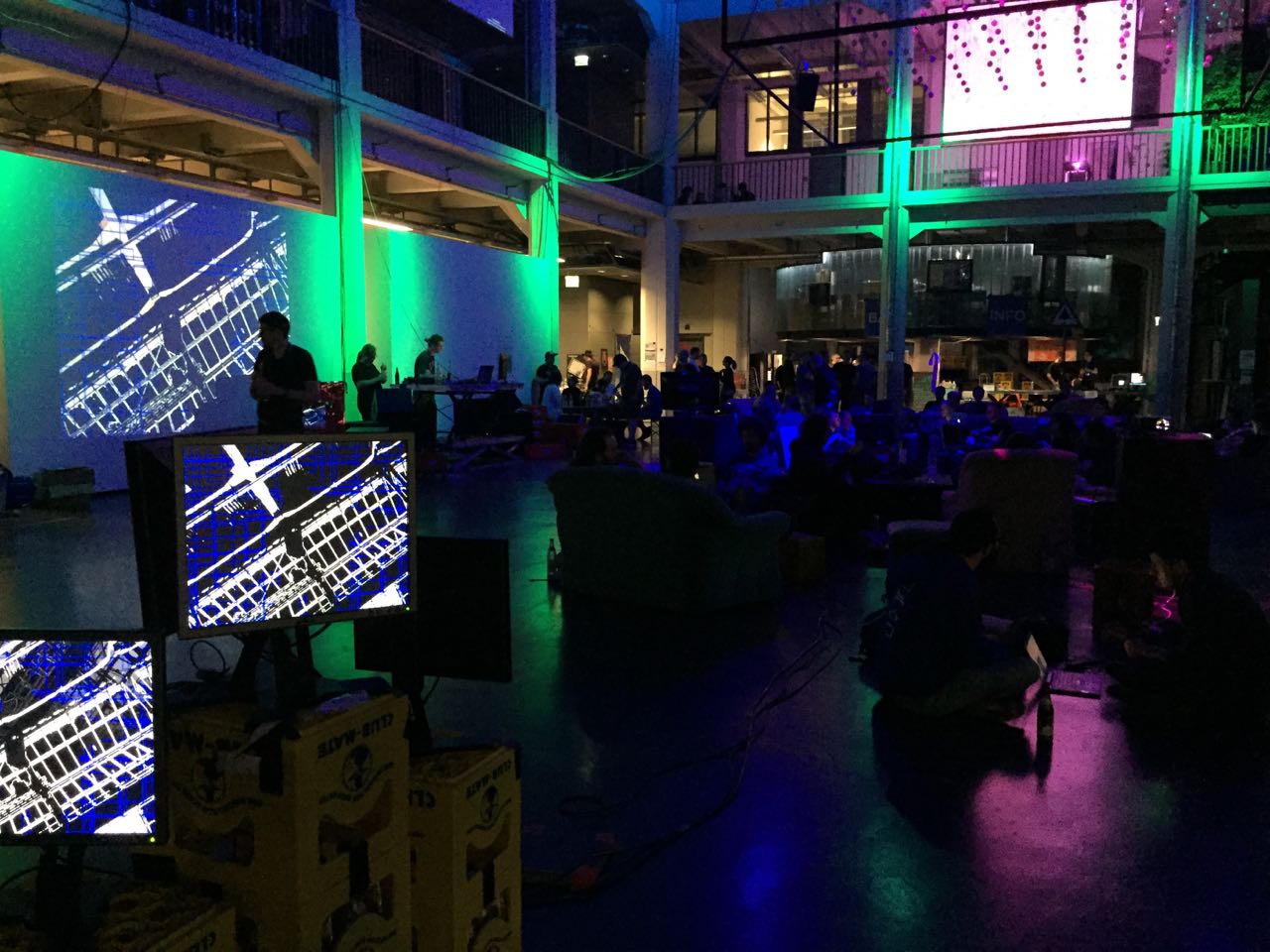
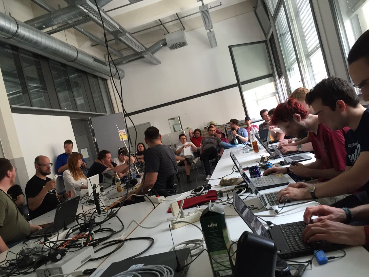
I spent the last weekend at the Gulasch Programmier Nacht (GPN) in Karlsruhe. Organized by the Chaos Computer Club (CCC), the GPN is an annual meeting of hackers and nerds, who meet to hang around, listen to talks, and eat Gulasch (goulash). I already read a lot about CCC events and finally made it to one. The people, the location, and the organization were really great.

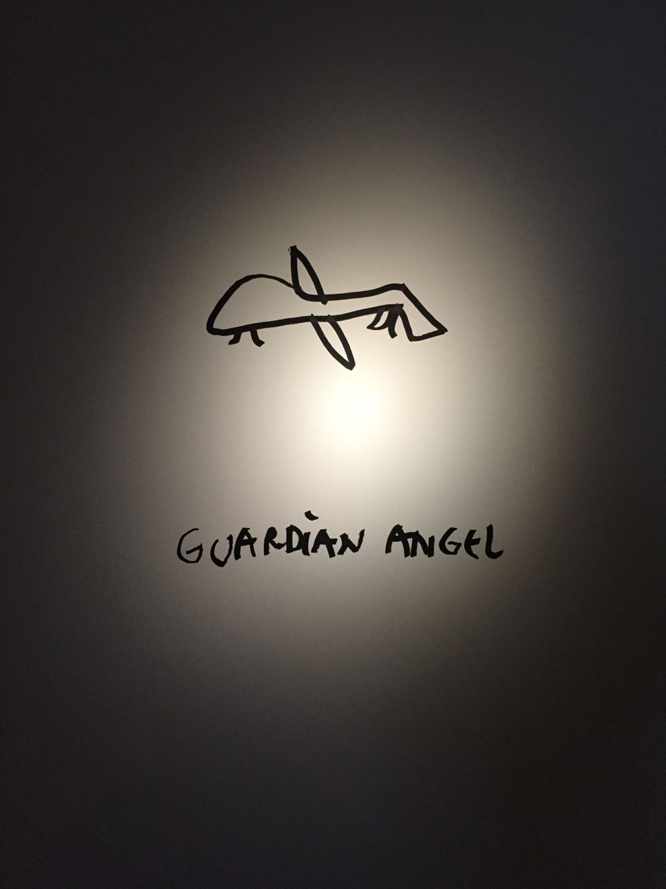
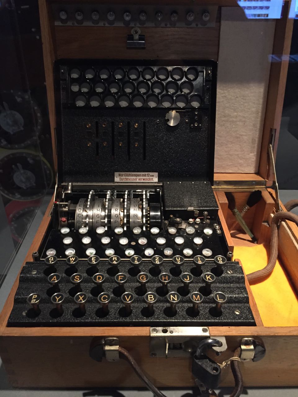
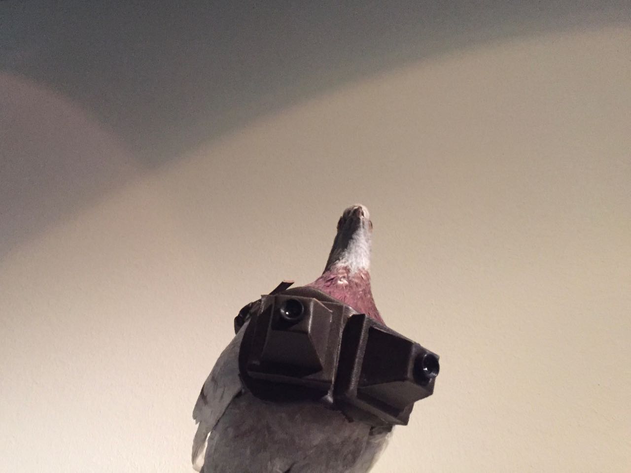
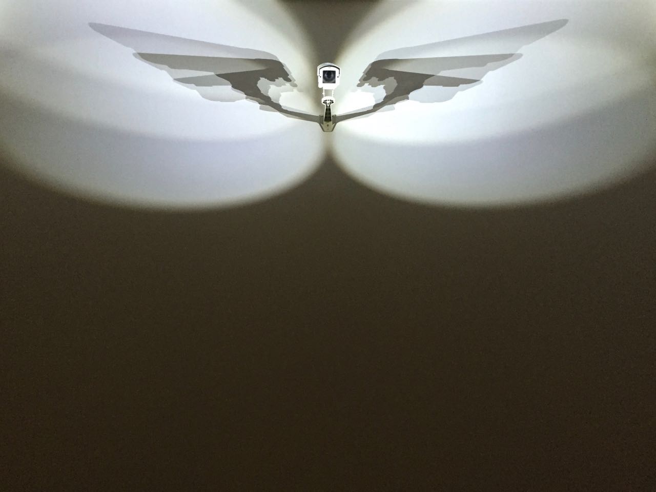
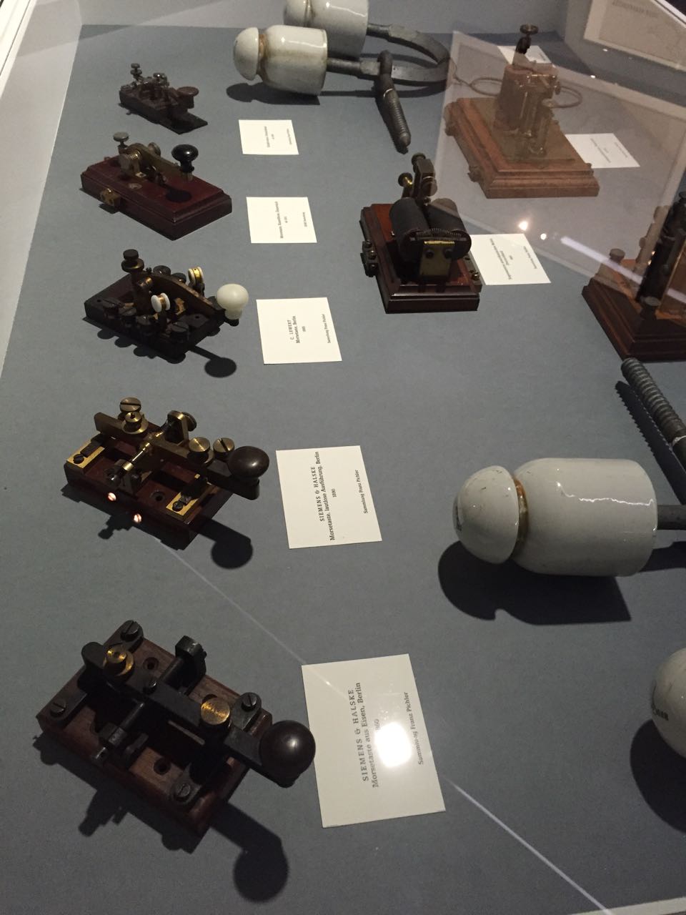
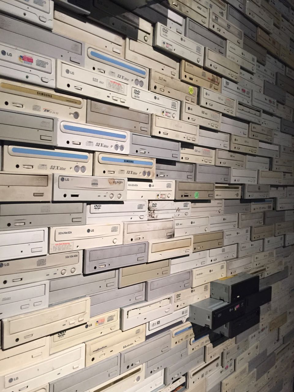
The GPN was hosted by the Zentrum für Kunst und Medientechnologie (ZKM), a high school for arts that has a museum attached. Currently, there’s a great exhibition about surveillance.

I’m very happy to be a Publication Co-Chair of IEEE Vehicular Networking Conference (VNC) 2016. This year’s iteration will be held in Columbus, Ohio, starting 8 December 2016. I heard being a publication chair can be a bit of a pain, but I’m looking forward to the new experience and the chance to serve the community :-)

I’m currently working on major updates to my GNU Radio WiFi Module. The goal is to make the module easier to extend with new algorithms, to make it more GNU Radio’ish and, finally, to get rid of the IT++ library.

As part of these updates I wanted to switch from demodulation with IT++ to GNU Radio’s constellation objects. Since there is no 64-QAM in GNU Radio and since the 16-QAM definition in gr-digital doesn’t match with what is defined for WiFi, I created my own constellations.

Turns out they are really cool and straightforward to use. In C++, I only had to define the complex constellation points and a decision maker that maps noisy samples to these constellation points. The whole magic for QPSK, for example, is something like:

constellation_qpsk_impl::constellation_qpsk_impl() {
    const float level = sqrt(float(0.5));
    d_constellation.resize(4);

    d_constellation[0] = gr_complex(-level, -level);
    d_constellation[1] = gr_complex( level, -level);
    d_constellation[2] = gr_complex(-level,  level);
    d_constellation[3] = gr_complex( level,  level);

    d_rotational_symmetry = 4;
    d_dimensionality = 1;
    calc_arity();
}

unsigned int
constellation_qpsk_impl::decision_maker(const gr_complex *sample) {
    return 2*(imag(*sample)>0) + (real(*sample)>0);
}

The tricky part is defining the SWIG bindings to make the constellations available in Python. I’m absolutely no SWIG expert, but I had the feeling that I had to work around some bugs or at least oddities of SWIG.

Obviously, I had to include the header that defines the abstract base class of constellation objects from gr-digital. The same header file, however, also contains the definitions of GNU Radio’s version of BPSK, QPSK, and 16-QAM. Actually, that shouldn’t be much of a problem since they are in different namespaces, but SWIG seems to mess that up.

So the first oddity is the need to explicitly ignore GNU Radio’s constellations when including the headers.

%ignore gr::digital::constellation_bpsk;
%ignore gr::digital::constellation_qpsk;
%ignore gr::digital::constellation_16qam;
%include "gnuradio/digital/constellation.h"

I’m very happy that my talk GQRX as a Graphical Frontend for Digital Receivers got accepted for the Software Defined Radio Academy, a workshop co-located with the HAMRADIO exhibition in Friedrichshafen.

The abstract goes like:

Developed by OZ9AEC, GQRX is a SDR with a graphical user interface that is very intuitive for radio amateurs. The waterfall plot, together with demodulators for FM, AM, and SSB, makes it a great tool for analog modes. GQRX is, however, not limited to analog transmissions, but is an excellent tool for digital modes too. Much like a conventional radio, it doesn’t aim to implement all digital modes internally, but provides means to export signals to audio files or stream them through network sockets. In this talk, we will show how this functionality allows to connect GQRX to other software, using it as a graphical frontend for various digital receivers. In particular, we will use a bit of format conversion to connect GQRX to multimon, custom GNU Radio receivers, and inspectrum, a new tool for offline signal analysis. Using the GUI of GQRX has the advantage that common functionality to find, filter, and demodulate a signal does not have to be reimplemented, allowing for rapid development of new receivers. Furthermore, the possibility to switch between storing and streaming data allows to develop offline receivers and later switch to live data seamlessly. I hope this talk gives some new ideas on how to get the most out of GQRX and how to combine it with other tools to ease receiver development.

This year’s program is again very interesting. Looking forward to Marcus Mueller’s introductory talk and Mike Walter’s talk about inspectrum, a new tool for offline signal analysis.

See you in Friedrichshafen.

Following up on my last posts, I wanted to point to Tim O’Shea’s recent work on GNU Radio channel models.

He looked into the flat fader block and came up with patches to fix problems regarding the autocorrelation, which I experienced earlier. With these changes, I’m very postivie that we have a validated and trustworthy fading implementation for GNU Radio.

In addition to that, he came up with a new tapped delay line channel model that introduces some randomness in the delay profile (usually only the amplitudes and phases of the individual paths change over time). So checkout his great post and watch the video.

The recordings of the Software Defined Radio Academy (SDRA), held in conjunction with HAMRADIO 2015, are now online.

I talked about reverse engineering wireless system using a wireless car key fob as an example.

Also be sure to check out Marcus Mueller’s introduction to GNU Radio and the reverse engineering talk from the guys from CCC Munich, who found public transportation signals on a digital subcarrier of FM broadcast radio.

<rant>

During the last weeks, I had my, by far, worst Open Source experience. While preparing simulations using GNU Radio’s Rayleigh fading block, I made some experiments to test its statistical properties. They showed some flaws, so I prepared patches and made a pull request.

The patches are already merged and should, at least, fix the most basic problems. Now, the block uses the correct number of sinusoids and outputs channel coefficients with an average power of one.

So far for so good. The point is that, in my opinion, there is still a non-trivial bug that corrupts autocorrelation properties. This is a bit of a problem as this model is basically all about generating channel coefficients with the proper autocorrelation.

OK, so I did the usual Open Source thing:

• Look at the documentation.
  It says that the block implements a basic fading model simulator that can be used to help evaluate, design, and test various signals, waveforms, and algorithms. OK.
• Look at the code.
  While the block mentions a Table 2, there is no reference where this table can be found. Since there are many, many ways to implement Rayleigh fading, it’s hard to fix without knowing what algorithm this is supposed to implement in the first place.

The Mailing List

The next step was, of course, to search the mailing list archives. At least I’m not the only one having problems with the block.

• Here, some guys conclude that the block does not work and should not be used. It didn’t trigger any comments/reactions from the developers; and usually they are pretty picky adding a for the record reply, even if others already came to a conclusion.
• Here, one of the developers experienced problems with the block. Of course he got a reply, but was pointed off-list. I asked for any new insights, but was ignored.
• OK, so I opened my own thread. It got completely ignored.
• A day later, another guy asked the same question. I tried to get a conversation going, but without much success.

Since nobody seemed to be interested I blogged about the problem. Just by looking at the graphs of the post, it should be easy to grasp that something is going wrong. I linked the post in the thread, hoping that now everybody should understand the problem. Still, no reaction from the developers.

I pushed the thread again and, this time, had a good conversation with another user. I think we brought the topic forward, and explicitly asked for feedback from the developers. Again, no reaction. I mean anything between simply stating that they are aware of our concerns and joining the discussion would have been OK. But nothing? Seriously?

Private Emails

I didn’t see any other option and wrote some core developers directly, asking if they could please comment on this thread. The reactions were something between I’m not interested; not my department; and no reaction at all. It’s now over a month since I submitted the first patches and I still have no clue what’s going on.

It’s OK, if someone doesn’t have the time or just doesn’t give a f!@#, but be mannered and tell other people who put considerable work into this shit!

</rant>

This IPython notebook generates channel coefficients with GNU Radio’s flat fader block and plots their autocorrelation at different points in time. The goal is to show how autocorrelation properties change, highlighting a potential bug in the model. See also the corresponding thread on the GNU Radio mailing list.

%matplotlib inline
import numpy as np
import matplotlib.pyplot as plt
plt.style.use('bmh')
plt.rcParams['figure.figsize'] = (10, 10.0*2/3)
plt.rcParams['font.size'] = 14
plt.rcParams['lines.linewidth'] = '3'


N = 12              # N sinusoids
v = 400 / 3.6       # speed (km/h to m/s)
f = 6e9             # freq
c = 3e8             # speed of light
f_d = f * v / c     # max. Doppler
samp_rate = 1e6     # 10 MHz
N_samp = int(1000 * samp_rate)  # samples to generate
fDTs = f * v / c / samp_rate
seed = np.random.randint(10000)

from gnuradio import gr, blocks, channels, analog
sig = analog.sig_source_c(0, analog.GR_CONST_WAVE, 0, 0, 1)
head = blocks.head(gr.sizeof_gr_complex*1, N_samp)
chan = channels.fading_model(N, fDTs, False, 4.0, seed)
snk = blocks.file_sink(gr.sizeof_gr_complex*1, "/home/basti/channel.bin", False)
snk.set_unbuffered(True)

## do simulations
tb = gr.top_block()
tb.connect(sig, head)
tb.connect(head, chan)
tb.connect(chan, snk)
tb.run()

In [3]:

import os

n_w = 4
w = int(n_w * c / f / v * samp_rate)

def autocorr(x, t=1):
    return np.corrcoef(np.array([x[0:len(x)-t], x[t:len(x)]]))

# resolution of autocorrelation
gaps = np.round(np.linspace(0, w, num=80))
gaps = gaps.astype(int)

## analytical
import scipy.special
bessel = map(lambda x: scipy.special.jv(0, 2 * np.pi * f_d / samp_rate * x), gaps)

N_items = 1000000

i = 0
while i < (N_samp - N_items):
    file = open("/home/basti/channel.bin", "rb")
    file.seek(i * 8, os.SEEK_SET)
    chan = np.fromfile(file, dtype=np.complex64, count=N_items)
    file.close()
    acorr = map(lambda x: np.abs(autocorr(chan, x)[0, 1]), gaps)
    
    fig, ax = plt.subplots()

    ax.plot(gaps/c*f*v/samp_rate, acorr, label='Simulations')
    ax.plot(gaps/c*f*v/samp_rate, np.abs(bessel), linestyle=':', label='Analytical')
    ax.axvline(0.4, linewidth=1, color='gray');
    ax.legend(loc=1)
    plt.show()
    
    i += 100000000

In [1]:

%matplotlib inline
import numpy as np
import matplotlib.pyplot as plt
plt.style.use('bmh')
plt.rcParams['figure.figsize'] = (18, 15)
plt.rcParams['font.size'] = 14
plt.rcParams['lines.linewidth'] = '3'

d_step = .1
fDTs = 1
N_samp = 1600
n = 0
d_theta = 0
d_N = 8

thetas = []
alphas = []
dopplers = []
coeffs = []
diffs = []

def update_theta():
    global d_theta
    global d_step
    d_theta += np.random.random() * d_step

    if (d_theta > np.pi):
        d_theta = np.pi
        d_step = -d_step
    elif (d_theta < -np.pi):
        d_theta = -np.pi
        d_step = -d_step


tmp = 0

for d_m in range(N_samp):
    alpha_n = (2*np.pi*n - np.pi + d_theta)/(4*d_N)
    doppler =      2*np.pi*fDTs*d_m*np.cos(alpha_n)
    coeff = np.cos(2*np.pi*fDTs*d_m*np.cos(alpha_n))

    diffs.append(doppler - tmp)
    tmp = doppler

    thetas.append(d_theta)
    alphas.append(alpha_n)
    dopplers.append(doppler)
    coeffs.append(coeff)
    update_theta()

fig, ax = plt.subplots(4, sharex=True)
fig.set_size_inches(18.5, 15.5)

ax[0].plot(thetas)
ax[0].set_title("d_theta")
ax[1].plot(alphas)
ax[1].set_title("alpha_n")
ax[2].plot(diffs)
ax[2].set_title("phase diff")
ax[3].plot(coeffs)
ax[3].set_title("coeff")
ax[3].set_xlabel("d_m (time)");

I was very happy to see that two of my last year’s projects are mentioned in the best of 2015 post of the RTL-SDR blog.

In August, they mention my project where I reverse engineered telemetry signals from public transportation

… and in September, they mention my reversing of signals from mobile traffic lights.

What a motivating start for 2016!